


Next: この文書について...
Up: 非線形離散値系
Previous: カオス現象
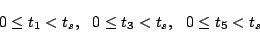
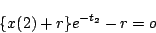
[例]プラントの伝達関数が次の場合、
出力:
 入力:
入力:
むだ時間:
サンプリング周期:
の無次元化および
を用いた制御方程式
図6.10より
 |
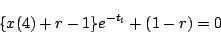
(6.6) |
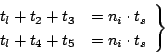 |
(6.7) |
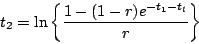
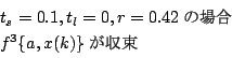
 の場合、初期値
 のとき
のとき
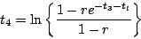
 |
(6.8) |
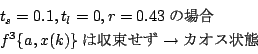
 の場合、初期値
 のとき
のとき
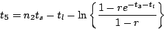
 |
(6.9) |
両式より
 |
(6.10) |
(6.7)式より
 |
(6.11) |
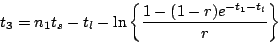
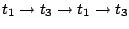
次の半周期は と
と を逆にして
を逆にして
 |
(6.12) |
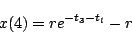
 |
(6.13) |
両式より
 |
(6.14) |
(6.7)式より
 |
(6.15) |
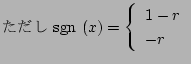
 は(6.6)式の条件を満足するように選ぶ。
 は次の周期の
 ゆえ、
ゆえ、
 を繰り返すことになる。
 は
は に相当
に相当
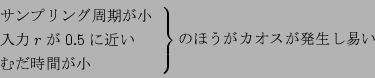
[例]
(a)
(b)
図 6.13:
vs. 
|
|
Next: この文書について...
Up: 非線形離散値系
Previous: カオス現象
Yasunari SHIDAMA
平成15年8月6日


![\includegraphics[scale=0.60]{eps/6-2-1.eps}](img43.png)
![\includegraphics[scale=0.60]{eps/6-2-2.eps}](img55.png)
![\includegraphics[scale=0.60]{eps/6-2-3.eps}](img77.png)
![\includegraphics[scale=0.60]{eps/6-2-4.eps}](img78.png)
![\includegraphics[scale=0.60]{eps/6-2-5.eps}](img83.png)