


Next: 可制御性、可観測性(Controllability,Observability)
Up: 状態方程式の性質
Previous: 状態方程式の性質
状態方程式
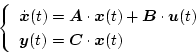 |
(2.98) |
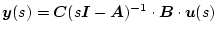
を初期値を としてラプラス変換すると、
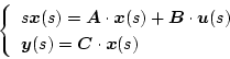 |
(2.99) |
となる。上式より
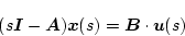 |
(2.100) |
となり、従って
| |
|
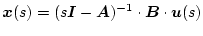 |
(2.101) |
| |
|
 |
(2.102) |
伝達関数行列は
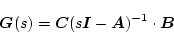 |
(2.103) |
となる。単入力・単出力システムのときは
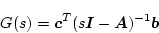 |
(2.104) |
となる。
 のすべての要素は分母が分子より1次以上高い
 の有理関数となる。
一般に有理関数行列
の有理関数となる。
一般に有理関数行列
 は
は
 がでない定数行列のとき
プロパ(proper)といい、
がでない定数行列のとき
プロパ(proper)といい、
 のとき厳密プロパ(strictly
proper)という。(2.103)式の形の
は常に後者となる。
のとき厳密プロパ(strictly
proper)という。(2.103)式の形の
は常に後者となる。
の分母は
 であるから
であるから
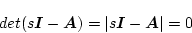 |
(2.105) |
が特性方程式となり、この式の根を固有値(特性根)という。
 例
例![$]$](img114.png)
![\begin{displaymath}
\left\{\begin{array}{l}
\dot{\mbox{\boldmath$x$}}=
\left[\be...
...1 & 0
\end{array}\right]\mbox{\boldmath$x$}
\end{array}\right.
\end{displaymath}](img228.png) |
(2.106) |
の場合
![$\mbox{\boldmath$A$}=
\left[\begin{array}{cc}
0 & 1\\
-2 & -3
\end{array}\right...
...ce{1cm}
\mbox{\boldmath$C$}^T=
\left[\begin{array}{cc}
1 & 0
\end{array}\right]$](img229.png)
ゆえ
| |
|
![$\displaystyle (s\mbox{\boldmath$I$}-\mbox{\boldmath$A$})=
\left[\begin{array}{c...
...end{array}\right]=
\left[\begin{array}{cc}
s & -1\\
2 & s+3
\end{array}\right]$](img230.png) |
(2.107) |
| |
|
 |
(2.108) |
| |
|
![$\displaystyle adj(s\mbox{\boldmath$I$}-\mbox{\boldmath$A$})=
\left[\begin{array}{cc}
s+3 & 1\\
-2 & s
\end{array}\right]$](img232.png) |
(2.109) |
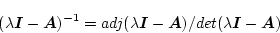
| |
|
![$\displaystyle (s\mbox{\boldmath$I$}-\mbox{\boldmath$A$})^{-1}=\frac{adj(s\mbox{...
...
\frac{\left[\begin{array}{cc}
s+3 & 1\\
-2 & s
\end{array}\right]}
{s^2+3s+2}$](img233.png) |
(2.110) |
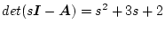
伝達関数は
になる。
特性方程式は
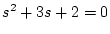
であり、固有値は および
および となる。
となる。
 |
(2.112) |
ゆえ
となり、
 の部分と
の部分と
 の
部分が交換可能であることがわかる。従ってどちらか一方がのとき
両者の積もとなる。
の
部分が交換可能であることがわかる。従ってどちらか一方がのとき
両者の積もとなる。
いま
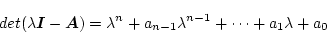 |
(2.114) |
とすると
 |
(2.115) |
になる。
 を代入すると
となり
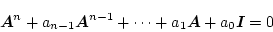 |
(2.117) |
になる。(2.117)式の関係をケーリー・ハミルトンの定理という。
前例の場合、 ゆえ
ゆえ
![$\left[\begin{array}{cc}
0 & 1\\
-2 & -3
\end{array}\right]^2+3
\left[\begin{ar...
...2
\end{array}\right]=
\left[\begin{array}{cc}
0 & 0\\
0 & 0
\end{array}\right]$](img254.png)
となり、同定理の成立することがわかる。
Next: 可制御性、可観測性(Controllability,Observability)
Up: 状態方程式の性質
Previous: 状態方程式の性質
Yasunari SHIDAMA
平成15年5月12日
![$\displaystyle \mbox{\boldmath$C$}^T(s\mbox{\boldmath$I$}-\mbox{\boldmath$A$})^{...
...s\end{array}\right]
\left[\begin{array}{c}0 1\end{array}\right]}
{s^2+3s+2}$](img235.png)
